The interplay of control and Deep Learning
It is superfluous to state the impact deep (machine) learning has had on modern technology, as it powers many tools of modern society, ranging from web searches to content filtering on social networks.
It is also increasingly present in consumer products such as cameras, smartphones and automobiles. Machine-learning systems are used to identify objects in images, transcribe speech into text, match news items, and select relevant results of search.
From a mathematical point of view however, a large number of the employed models and techniques remain rather ad hoc.
1 Formulation
When formulated mathematically, deep supervised learning [1,3] roughly consists in solving an optimal control problem for a nonlinear dynamical system, called an artificial neural network. We are interested in approximating a function:
f: \R^d \rightarrow \R^mof some class, which is unknown a priori.
We have data: its values (possibly noisy) at S distinct points:
\{\vec{x}_i, \vec{y}_i = f(\vec{x}_i) \}_{i=1}^SWe generally split the S data points into N training data, and S−N−1 test data. In practice, N is significantly bigger than S −N −1. “Learning” generally consists in:
1. Proposing a candidate approximation:
f_{A,b}(\cdot): \R^d \rightarrow \R^mdepending on tunable parameters (A,b). A popular candidate for such a function is (a projecton of) the solution zi(1) of a neural network, which in the simplest continuous-time context reads:
\begin{cases} z_i'(t) &= \sigma(A(t)z_i(t)+b(t)) \quad \text{ in } (0, 1) \\ z_i(0) &= \vec{x}_i \in \R^d. \end{cases}
2. Tune (A,b) as to minimize the empirical risk:
\sum_{i=1}^N \ell(f_{A,b}(\vec{x}_i), \vec{y}_i), \quad \ell \geq 0, \,\ell(x, x) = 0.This is called training. As generally N is rather large, the minimizer is computed via an iterative method such as stochastic gradient descent (Robbins-Monro [7], Bottou et al [8]).
3. A posteriori analysis: check if test error
\sum_{i=N+1}^{S} \ell(f_{A,b}(\vec{x}_i), \vec{y}_i)is small
This is called generalization. In the above, σ is a fixed, non-decreasing Lipschitz-continuous activation function.
• There are two types of tasks in supervised learning: classification (labels take values in a discrete set), and regression(labels take continuous values).
• In practice, one generally considers the corresponding discretisation of the continuous-time dynamical system given above.
• The simplest forward Euler discretisation of the above system is called a residual neural network(ResNet) with L hidden layers:
\begin{cases} z_i^{k+1} = z_i^k + \sigma(A^k z_i^k + b^k) &\text{ for } k = 0, \ldots, L-1 \\ z_i^0 = \vec{x}_i \in \R^d. \end{cases}
2 Optimal control
Summarizing the preceding discussion, in a variety of simple scenarios, deep learning may be formulated as a continuous-time optimal control problem:
\inf_{u(t) \in U,\, (\alpha, \beta)} \sum_{i=1}^N |\vec{y}_i - \varphi(\alpha \, z(1)+\beta)|^2 + \frac{\epsilon}{2} \int_0^1 |(A(t), b(t))|^2 dtwhere z = z_i solves
\begin{cases} z'(t) &= \sigma(A(t)z(t)+b(t)) \quad \text{ in } (0, 1) \\ z(0) &= \vec{x}_i \in \R^d. \end{cases}The idea of viewing deep learning as finite dimensional optimal control is (mathematically) formulated in [9], and subsequently investigated from a theoretical and computational viewpoint in [5, 6, 7, 8], among others.
Figure 2. The time-steps play the role of layers. We see that the points are linearly separable at the final time. Movie of the evolution of the trajectories. See [10]
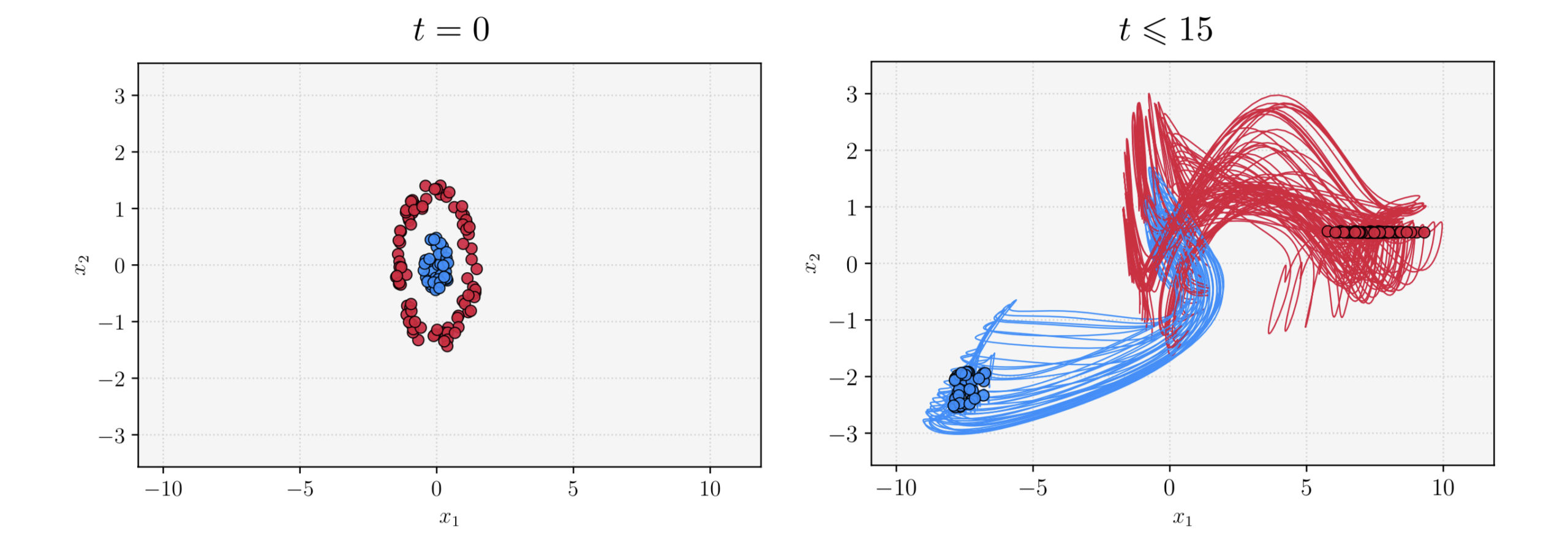
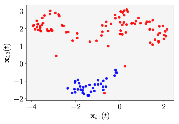
Figure 3. A batch of training data (left) and the evolution of the corresponding trained trajectories xT,i(t) (right) in the phase plane. The learned flow is simple, with moderate vari- ations, due to the exponentially small parameters. See [10]
It is at the point of generalisation where the objective of supervised learning differs slightly from classical optimal control.
Indeed, whilst in deep learning one too is interested in “matching” the labels of the training set, one also needs to guarantee satisfactory performance on points outside of the training set.
Our goal
The work of our team consists in gaining a better understanding of deep supervised learning by merging the latter with well-known subfields of mathematical control theory and numerical analysis.
References
[1] Ian Goodfellow and Yoshua Bengio and Aaron Courville. (2016). Deep Learning, MIT Press
|| Go to the Math & Research main page